Hyper Diffusion Planner

Unleashing the Potential of Diffusion Models
for End-to-End Autonomous Driving

Yinan Zheng*†,1, Tianyi Tan*1, Bin Huang*2, Enguang Liu2, Ruiming Liang1, Jianlin Zhang2, Jianwei Cui2, Guang Chen2, Kun Ma2, Hangjun Ye2, Long Chen2, Ya-Qin Zhang1, Xianyuan Zhan✉,1, Jingjing Liu✉,1
1Institute for AI Industry Research (AIR), Tsinghua University  ·  2Xiaomi EV
*Equal contribution    ✉Corresponding author    †Project Lead
HDP Framework Overview

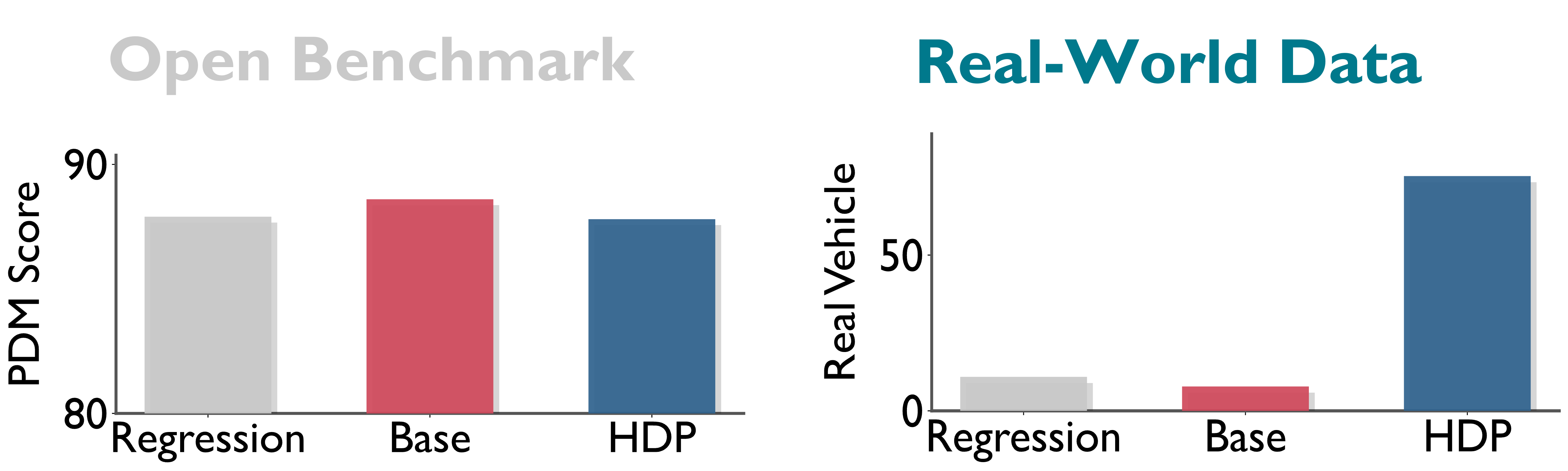
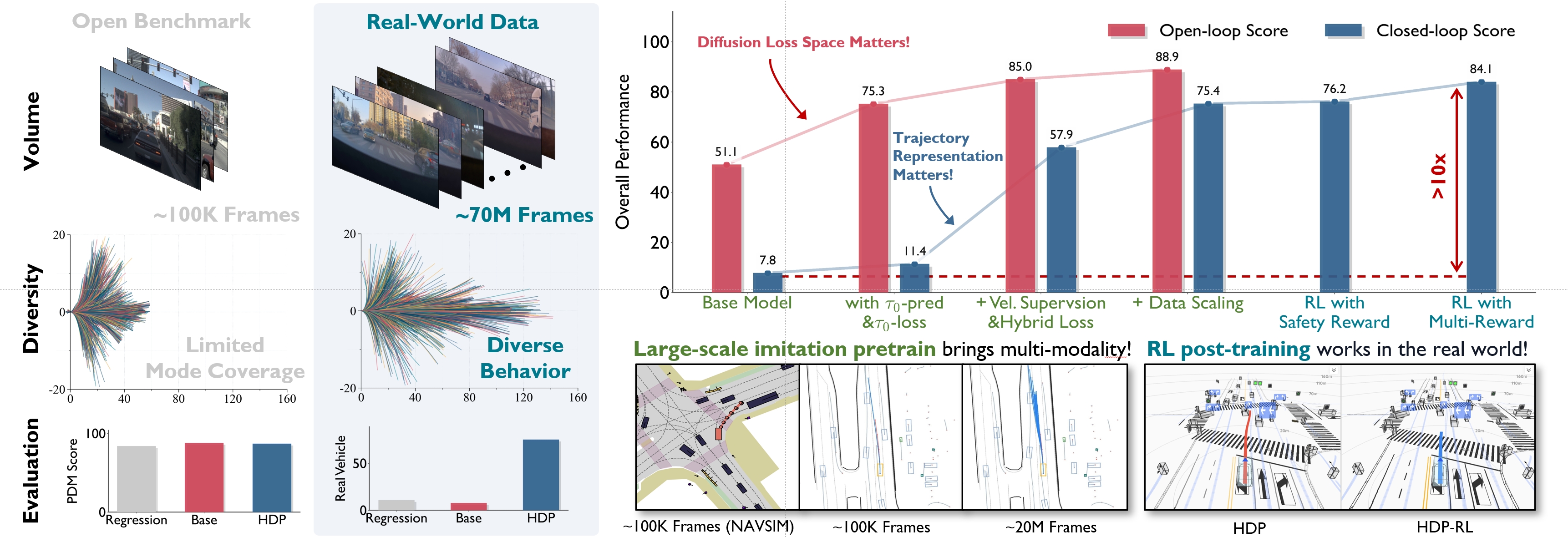
Simulation-based benchmarks differ substantially from real-world deployment, leaving the true capability of diffusion-based planners largely unverified. Through a detailed investigation of the IL/RL training recipe, we unleash the potential of diffusion-based planning, achieving a 10x improvement in real world.

Abstract

Diffusion models have become a popular choice for decision-making tasks in robotics, and more recently, are also being considered for solving autonomous driving tasks. However, their applications and evaluations in autonomous driving remain limited to simulation-based or laboratory settings. The full strength of diffusion models for large-scale, complex real-world settings, such as End-to-End Autonomous Driving (E2E AD), remains underexplored. In this study, we conducted a systematic and large-scale investigation to unleash the potential of the diffusion models as planners for E2E AD, based on a tremendous amount of real-vehicle data and road testing. Through comprehensive and carefully controlled studies, we identify key insights into the diffusion loss space, trajectory representation, and data scaling that significantly impact E2E planning performance. Moreover, we also provide an effective reinforcement learning post-training strategy to further enhance the safety and robustness of the learned planner. The resulting diffusion-based learning framework, Hyper Diffusion Planner (HDP), is deployed on a real-vehicle platform and evaluated across 6 urban driving scenarios and 200 km of real-world testing, achieving a notable 10x performance improvement over the base model. Our work demonstrates that diffusion models, when properly designed and trained, can serve as effective and scalable E2E AD planners for complex, real-world autonomous driving tasks.

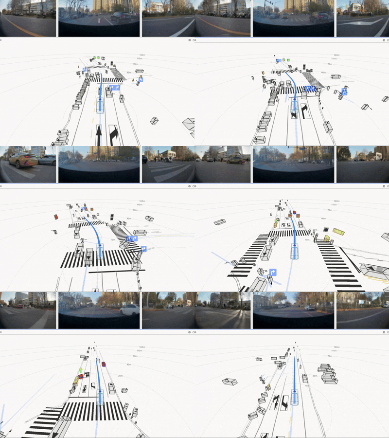
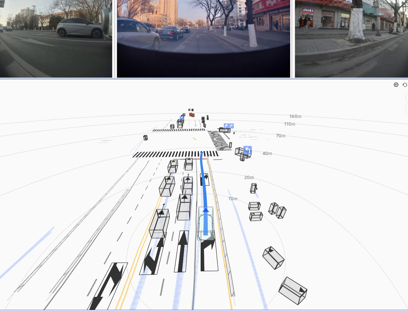
Demo 1
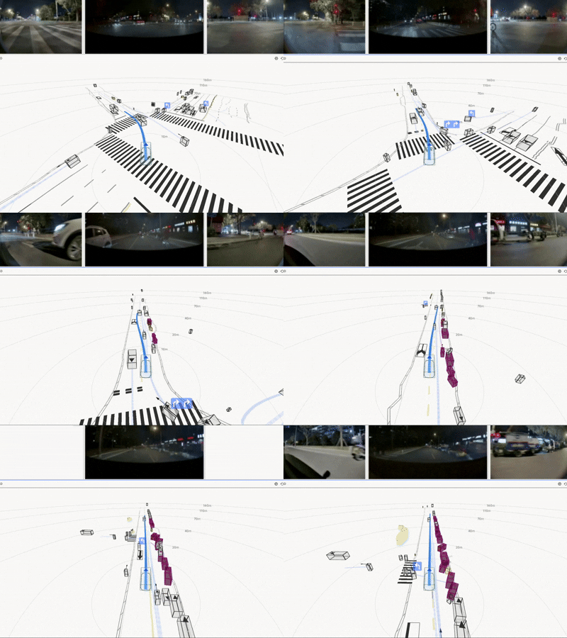
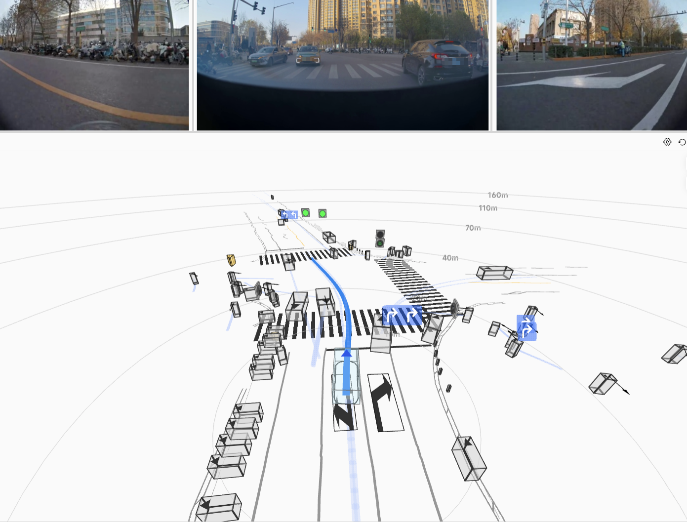
Demo 2
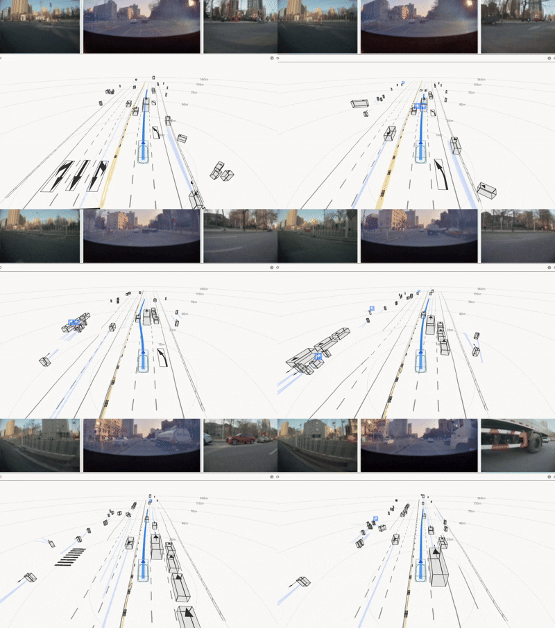
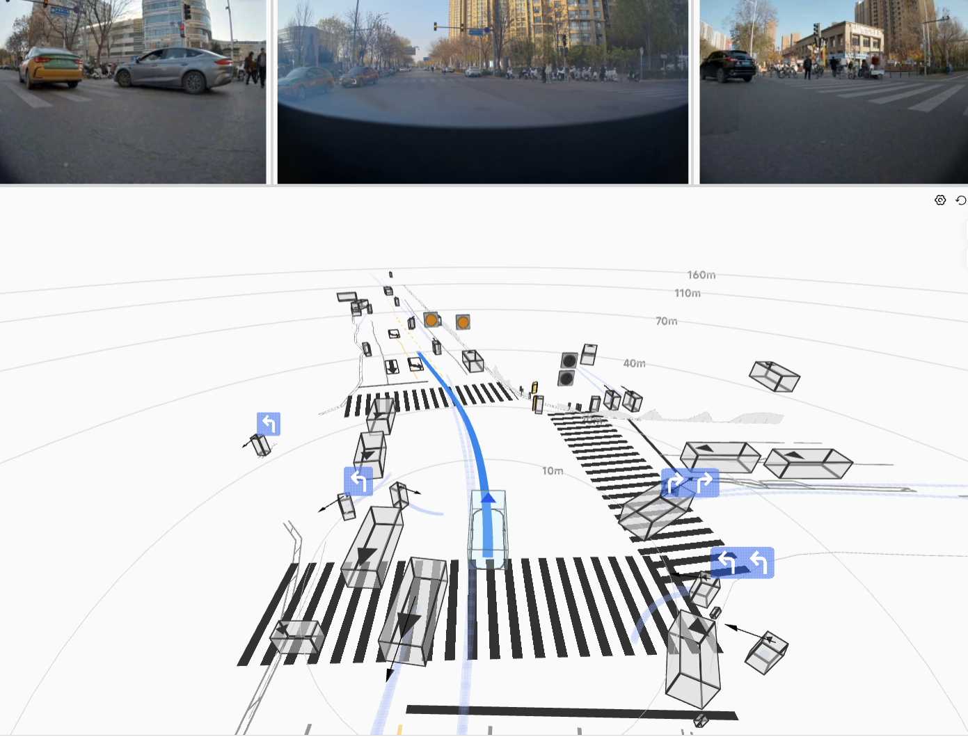
Demo 3

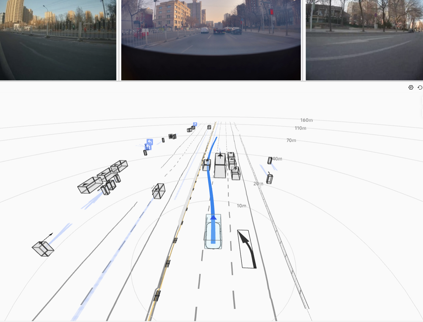
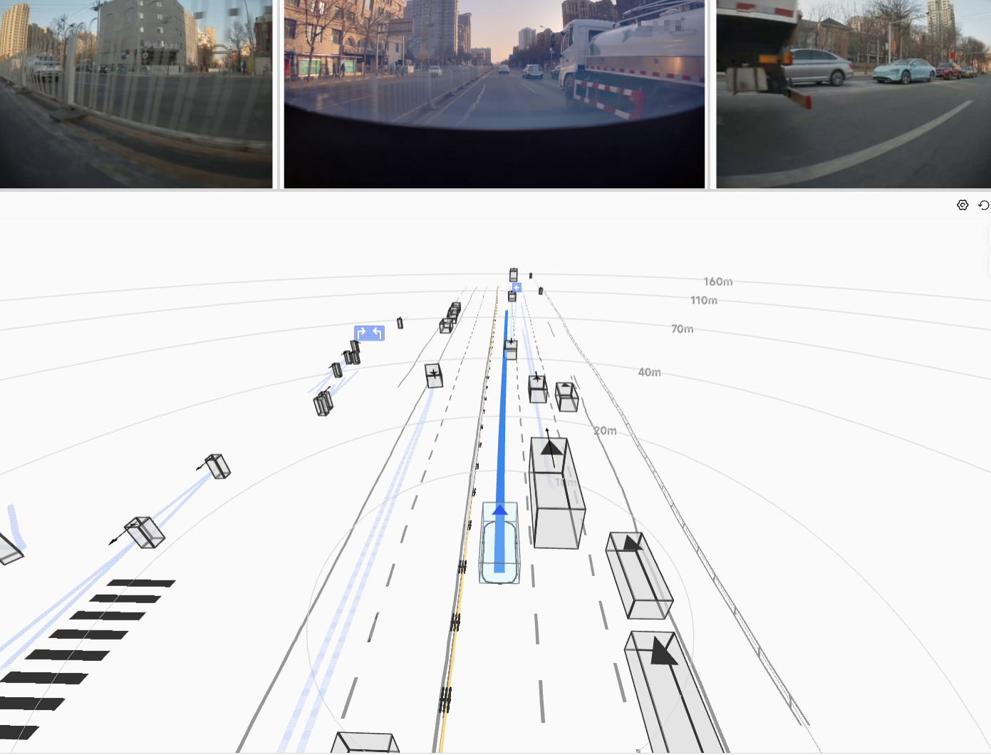
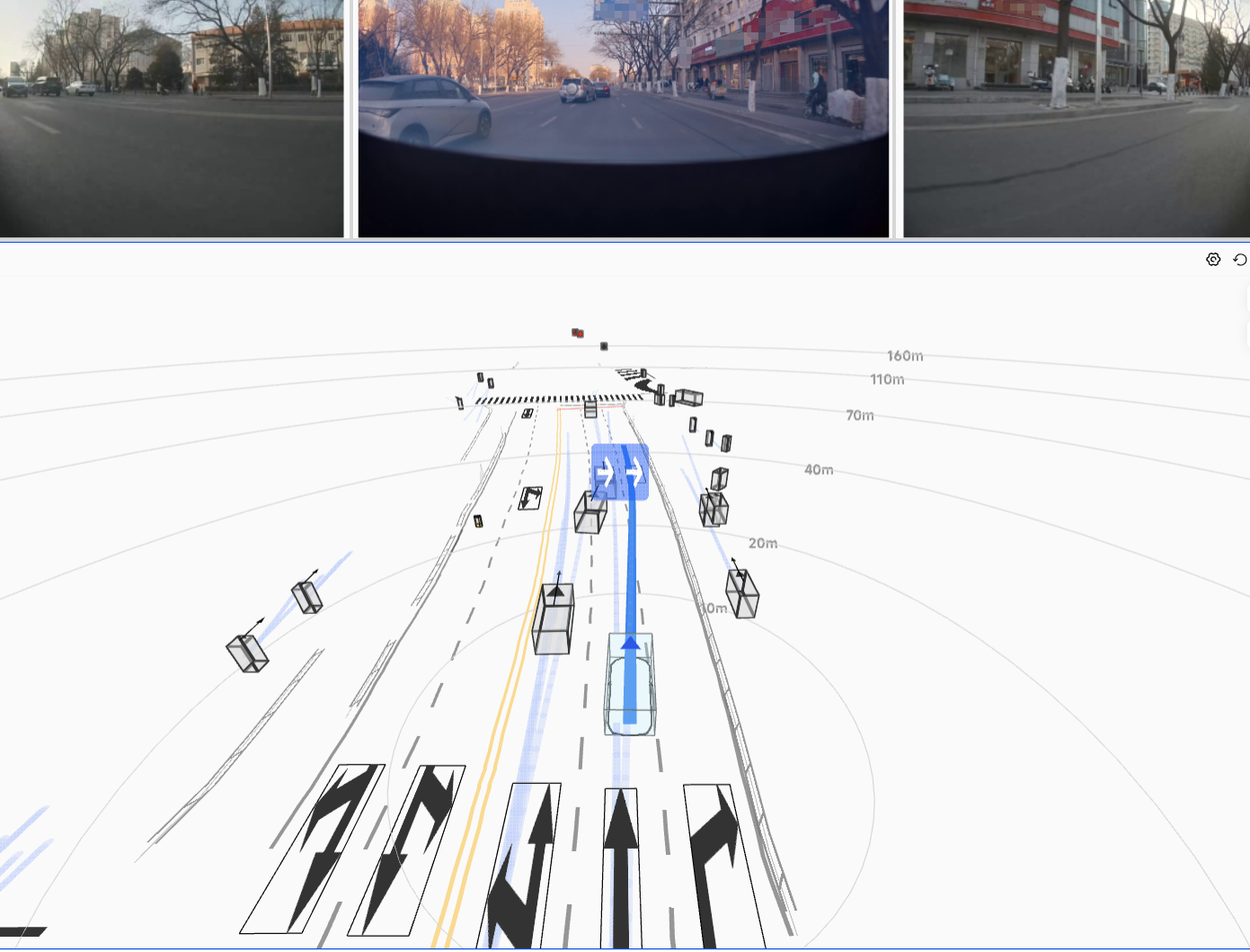
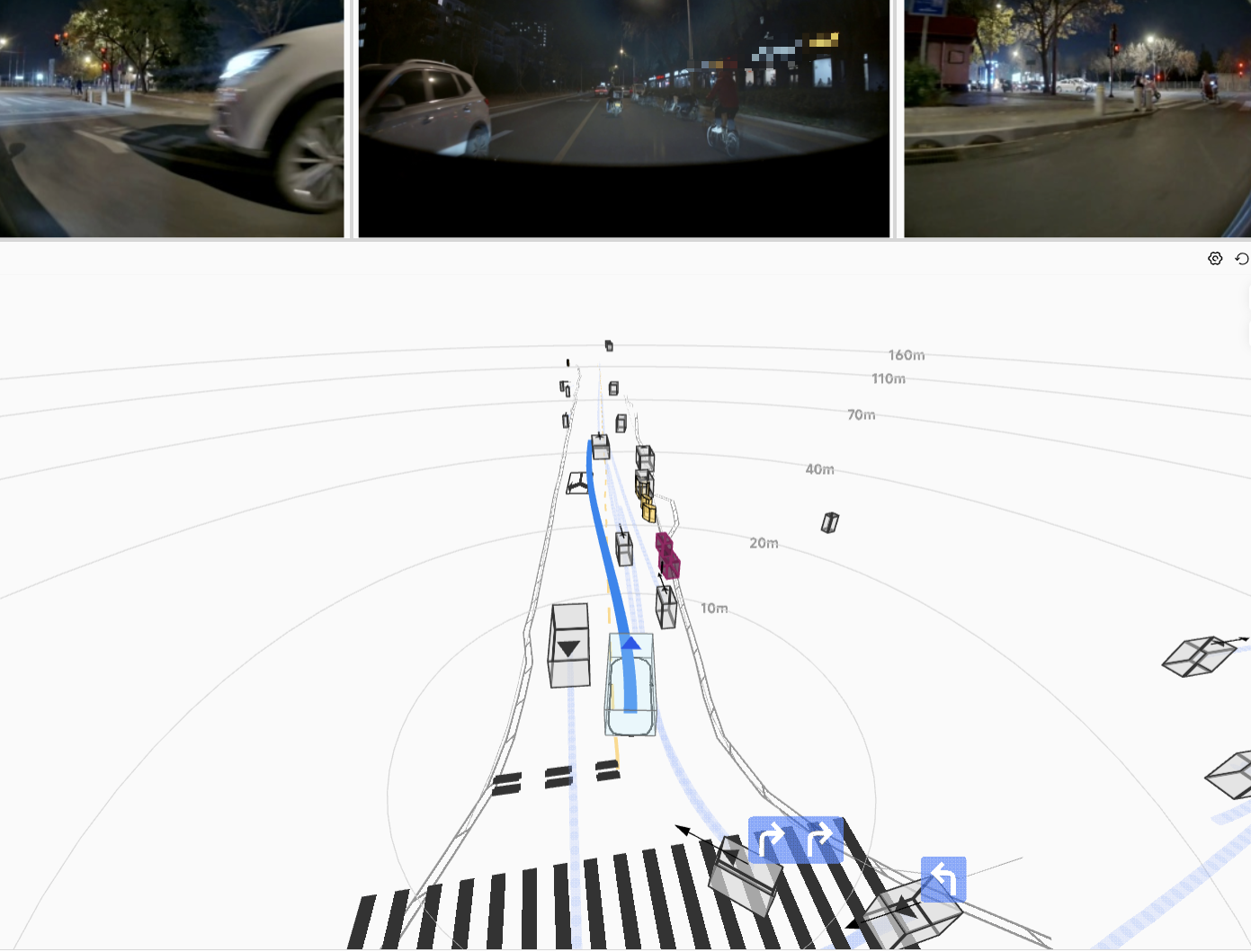
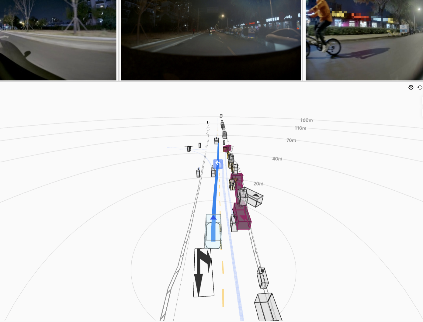
Real-world urban driving — model output with only minimal smoothness post-refinement.

When Benchmark Meets Reality

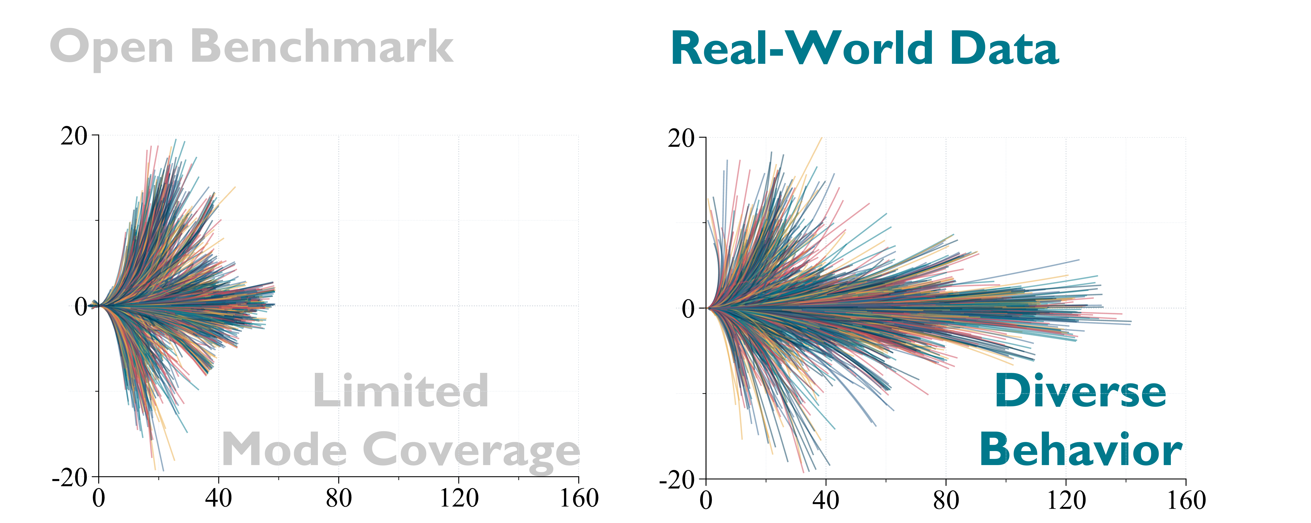
Public benchmarks have substantially advanced end-to-end autonomous driving, yet a central question remains: to what extent do benchmark scores reflect real-world driving capability? In practice, the gap between benchmark evaluation and deployment persists along three dimensions:

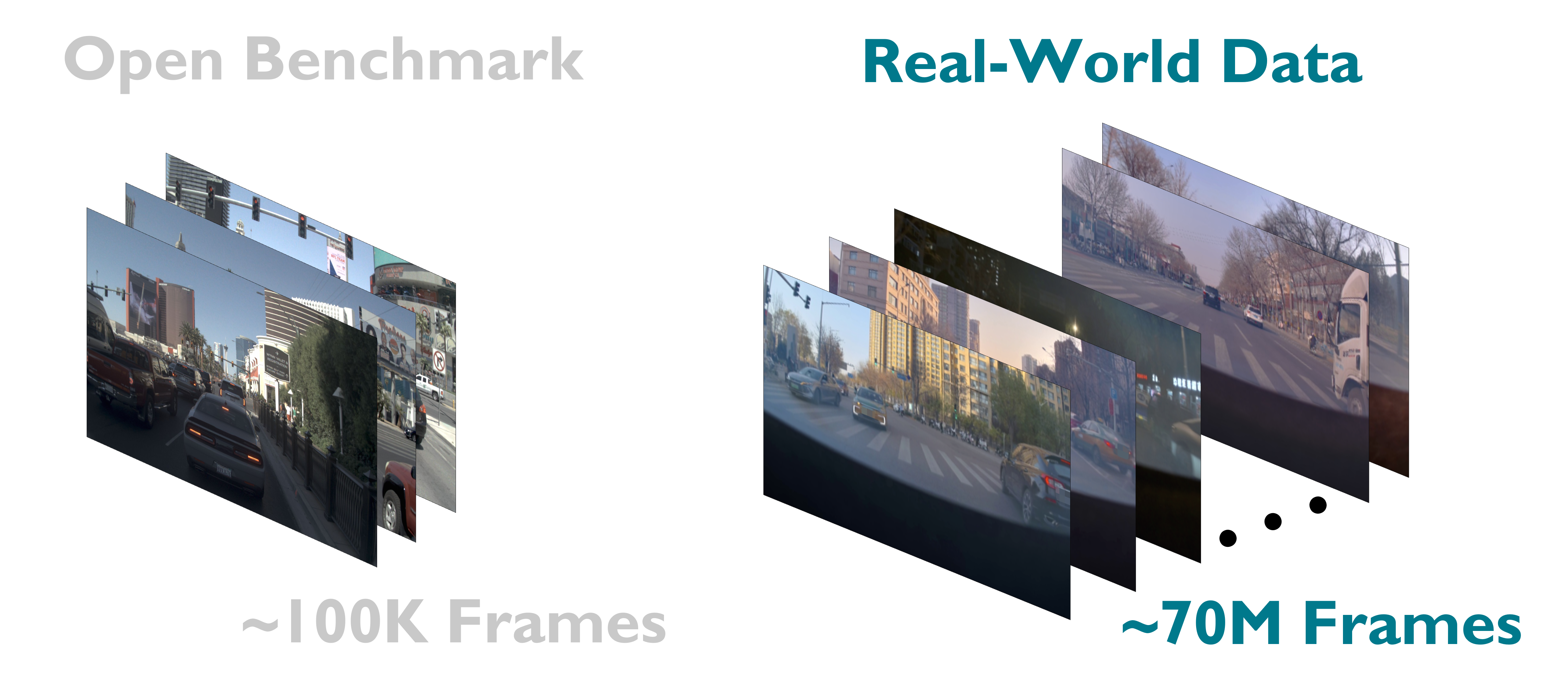
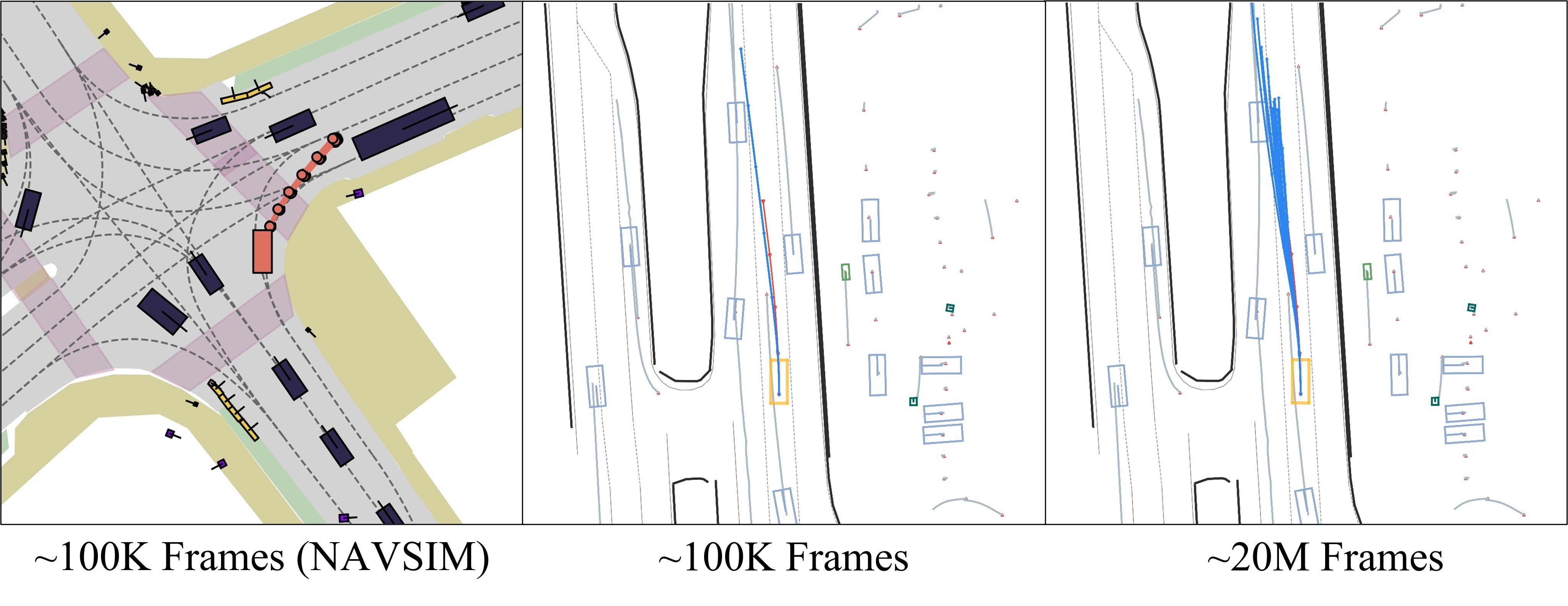
Scale Gap. Benchmark scale remains far below that of real-world training.
Diversity Gap. Benchmark diversity remains substantially narrower than real traffic.
Evaluation Gap. Pseudo closed-loop evaluation remains an proxy for real-vehicle End-to-End AD.
Scale gap illustration
Coverage gap illustration
Evaluation gap illustration

Taken together, these gaps suggest that benchmark success should not be conflated with real-world driving competence. Faithful assessment requires large-scale real-world data and rigorous closed-loop validation.

Method

We systematically study four key design axes to unleash the full potential of diffusion-based planning for real-world autonomous driving.

1 — Rethinking Diffusion Loss Space

Diffusion models are typically trained to predict one of three quantities: the clean data τ0, the noise ε, or the flow velocity v. These targets are mathematically inter-convertible, yet they induce very different learning dynamics. Since existing configurations are inherited from image generation—a domain fundamentally different from planning—we revisit the choice by evaluating all 9 prediction–loss combinations on our planning task.

Key finding: τ0-prediction with τ0-loss converges the fastest, generates the smoothest trajectories, and provides the best manifold coverage. The ε-prediction models, by contrast, suffer from high-frequency jitter and even complete breakdown under certain loss pairings.

Why? The trajectory τ0 lives on a low-dimensional manifold that the network can fit directly, while ε and v targets occupy much higher-dimensional spaces that demand greater capacity and exhibit training instability. In particular, τ0-prediction demonstrates superior stability during the final low-noise denoising steps, effectively suppressing high-frequency artifacts to yield kinematically coherent trajectories. Getting this "training coordinate system" right is the prerequisite for all subsequent improvements.

Training curves

The learning curve of models trained with different loss designs.

Trajectory quality grid

The open-loop visualization of planning trajectories.

2 — Hybrid Trajectory Representation

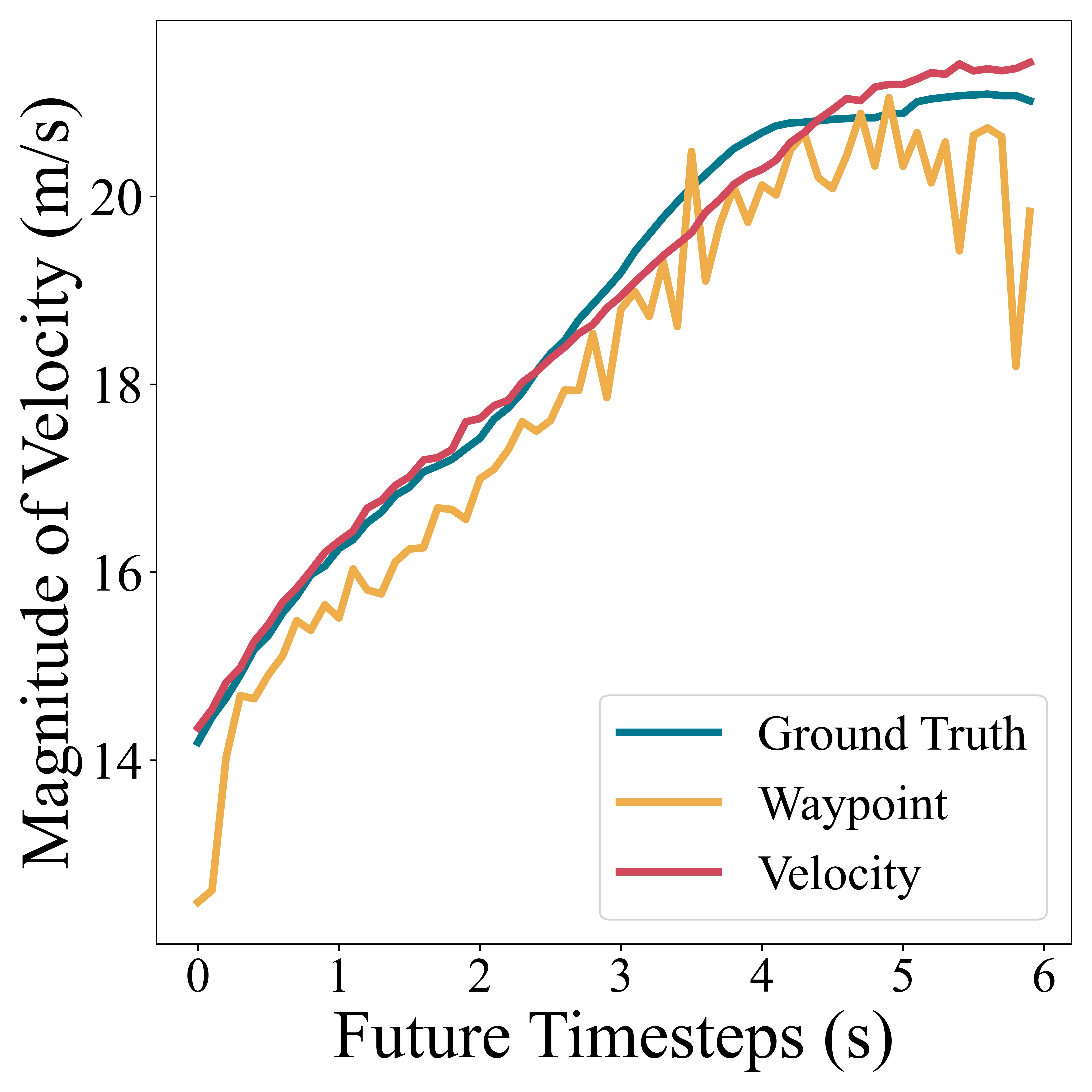
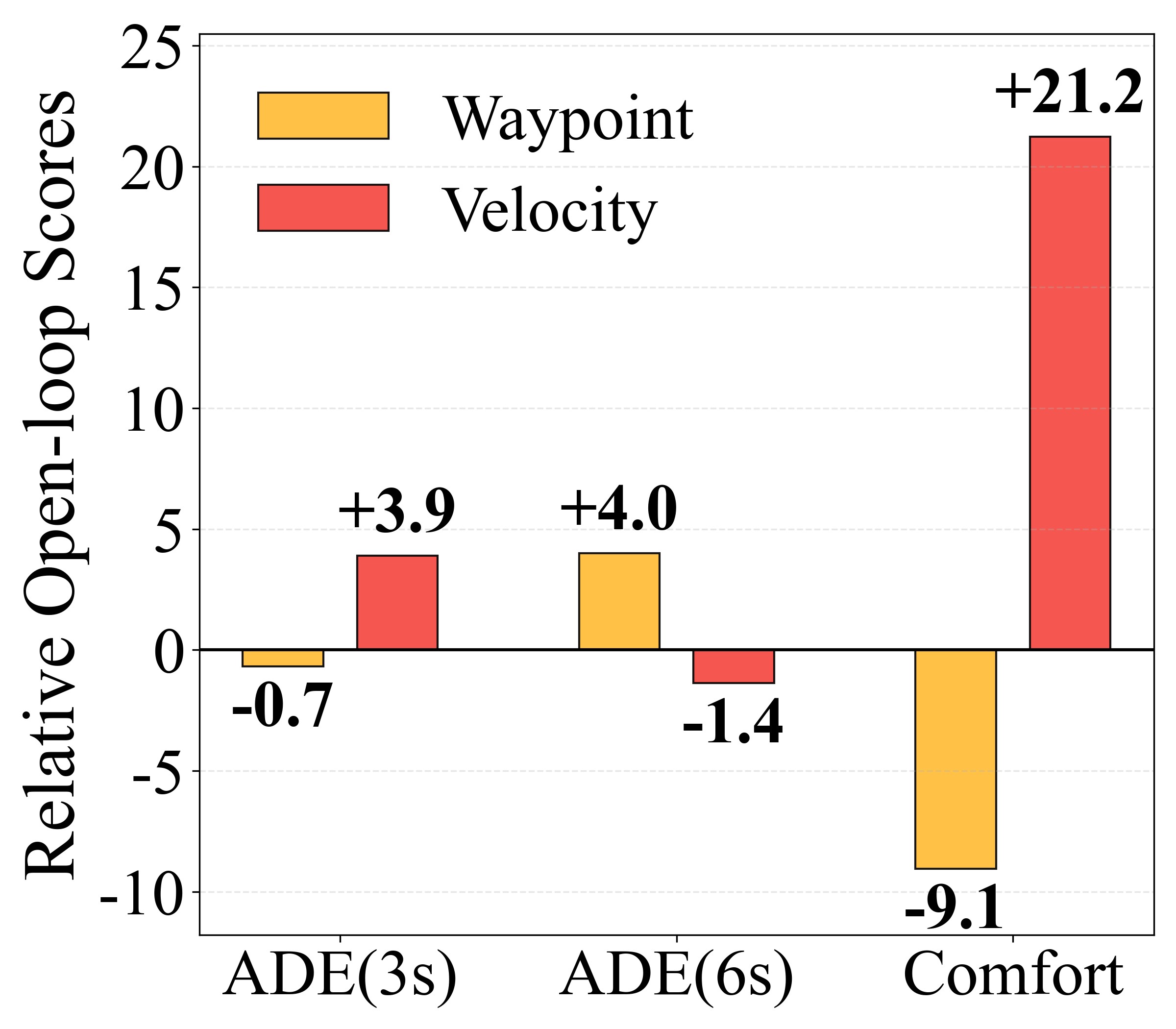
With τ0-prediction established, a problem emerges when inspecting higher-order statistics: waypoint trajectories capture global geometry well but produce jerky velocity profiles, while velocity trajectories are kinematically smooth yet sacrifice geometric accuracy. Choosing only one forces an undesirable trade-off.

Our solution — Hybrid Loss: The model outputs velocity for numerical stability, but training jointly supervises both the velocity error and the integrated-waypoint error, combining the geometric strength of waypoints with the kinematic smoothness of velocity.

Theoretical guarantee: We prove that the Hybrid Loss is equivalent to a score-matching loss under a positive-definite weighted P-norm, ensuring the learned score function remains unbiased.

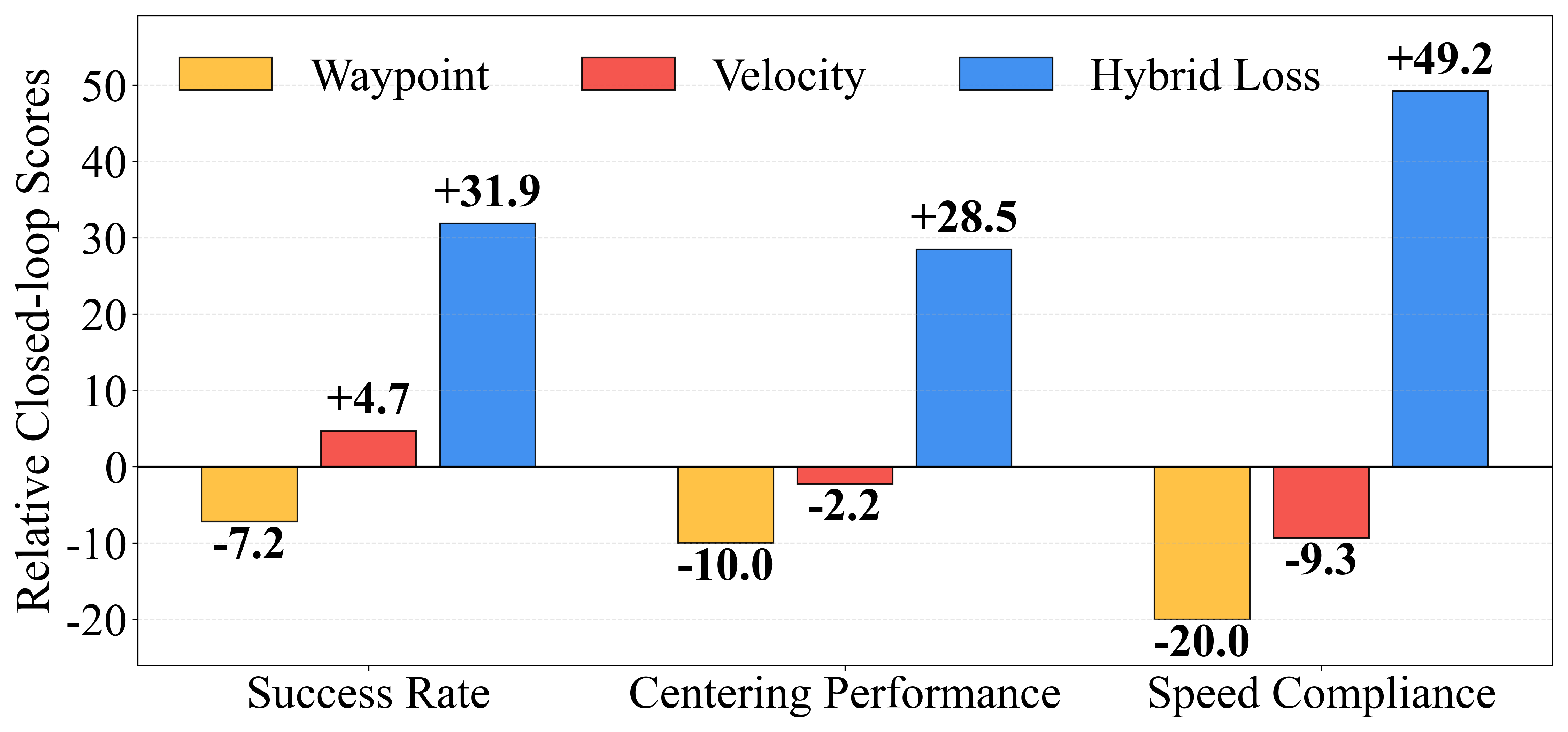
Real-vehicle performance: In closed-loop tests, the Hybrid Loss substantially improves both success rate and comfort over single-representation baselines—the critical step from "it drives" to "it drives well."

v-t curve Metrics comparison

Left: vt curves—waypoints jitter, velocity is smooth. Right: Metric comparison.

Hybrid loss gains

Closed-loop results: Hybrid Loss outperforms both single-representation baselines across all metrics.

Theorem — Hybrid loss = score matching under P-norm

The Hybrid Loss can be equivalently rewritten as a weighted score-matching objective:

$\mathcal{L}_{\text{hybrid}} \;=\; \mathbb{E}_{\tau^{\mathbf{v}}_{0},\,\epsilon,\,t}\!\left[\,\lVert \tau^{\mathbf{v}}_{\theta} - \tau^{\mathbf{v}}_{0} \rVert_{\mathit{P}}^{2}\,\right]$

where $\mathit{P} = I + \Delta t^{2}\,\omega\, M^{\!\top}\!M$ is positive-definite. By Bregman-divergence theory, this quadratic objective is a valid score-matching loss whose unique minimizer is $\mathbb{E}[\tau^{\mathbf{v}}_{0}\mid\tau^{\mathbf{v}}_{t}]$ — recovering the marginal score function. Integrating velocity into waypoint supervision therefore introduces no bias to the diffusion model.

Remark 1 — Generality of M

The proof only requires $M^{\!\top}\!M \succeq 0$, which holds for any matrix $M$. The lower-triangular integration matrix is just the physically meaningful choice we adopt; other kinematic couplings (e.g. acceleration) remain valid score-matching objectives.

Remark 2 — Why not $L_1$ or auxiliary planning losses

$L_1$-norm losses (e.g. DiffusionDrive) and prediction-dependent auxiliary losses (e.g. VAD collision loss) are not Bregman divergences. Their minimizers do not coincide with $\mathbb{E}[\tau^{\mathbf{v}}_{0}\mid\tau^{\mathbf{v}}_{t}]$, yielding biased score estimators.

Algorithm 1 — Hybrid loss with detached integral

def detached_integral(v, W, dt):
    # v : velocity of future trajectory
    # W : gradient detach window size
    # dt: time interval
    wpt_sg   = torch.cumsum(v.detach()) * dt
    shift_sg = torch.roll(wpt_sg, shifts=W)
    shift_sg[:W] = 0

    wpt   = torch.cumsum(v) * dt
    shift = torch.roll(wpt, shifts=W)
    shift[:W] = 0

    return wpt + shift_sg - shift


def hybrid_loss(pred_v, gt_v, W, omega):
    # omega : loss balancing weight
    l_v   = (pred_v - gt_v) ** 2
    l_wpt = (detached_integral(pred_v, W, dt)
             - torch.cumsum(gt_v) * dt) ** 2
    return l_v + omega * l_wpt

The detached integral restricts gradient backpropagation to a temporal window of $W$ steps, rebalancing supervision across future timesteps without altering the loss minimizer.

3 — Data Scaling & Emergent Multimodality

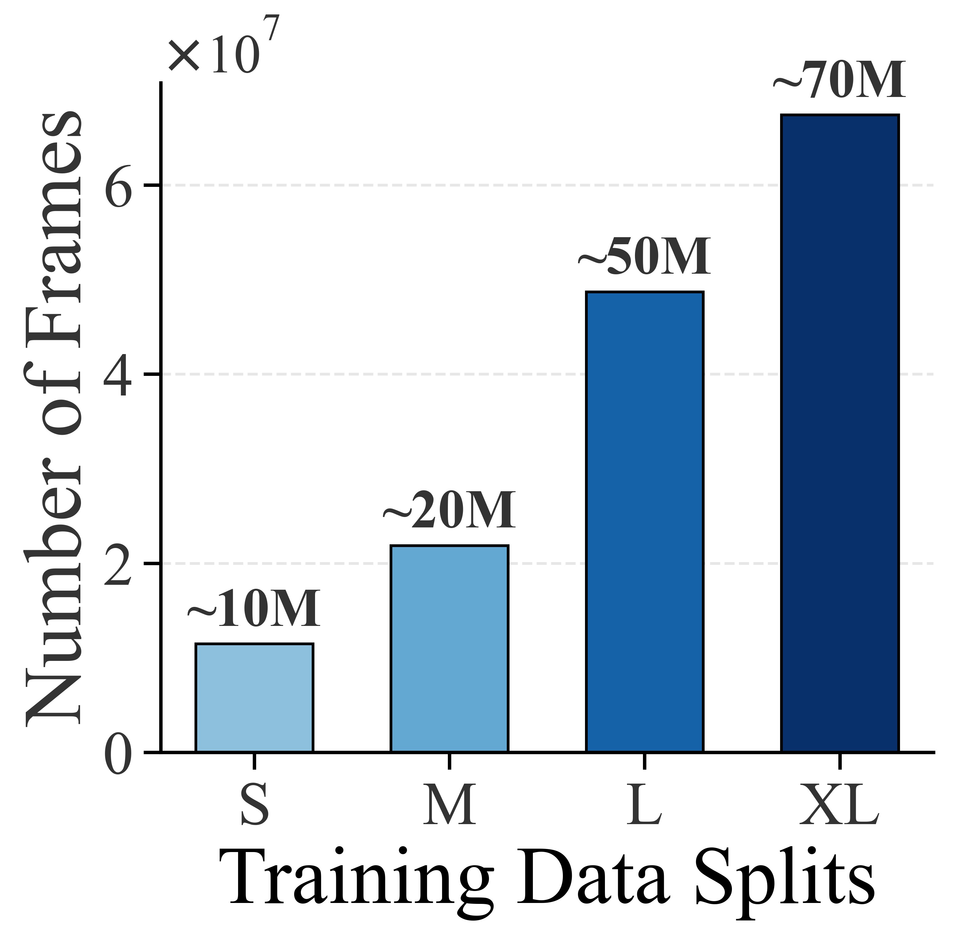
Diffusion models are renowned for multimodal generation, yet existing AD benchmarks (e.g., NAVSIM with only ~100K frames) are far too small to exhibit this capability, leading to severe mode collapse. To investigate, we conduct controlled experiments scaling real-vehicle data from 100K to 70M frames—orders of magnitude beyond typical academic settings.

Key finding: At 100K frames the model collapses to a single mode. As data grows past 1M, multimodal behavior emerges—the trajectory divergence score increases steadily. Both open- and closed-loop metrics improve continuously, with 20%+ closed-loop gain from 10M to 70M alone.

This validates that a clean diffusion planning architecture, free of anchors or goal conditioning, can effectively exploit industrial-scale data—consistent with the theoretical result that diffusion models need sufficient training data for generalization.

Scaling curve Multimodal

Left: Trajectory divergence vs. data size—multimodality emerges with scale. Right: All trajectories collapse at 100K; diverse modes at 20M.

Data splits Performance scaling

Left: Training data splits (S / M / L / XL). Right: Both open- and closed-loop performance scale steadily with data.

4 — RL Post-Training

Imitation learning produces a strong behavioral prior but provides no explicit safety constraint—a critical gap for deployment. We close it with an RL post-training stage that directly optimizes a safety-aware reward while keeping the entire diffusion architecture intact.

We formulate a KL-regularized policy optimization objective that constrains the updated policy to stay close to the referece policy. Its closed-form solution is an elegant reward-reweighting: the existing Hybrid Loss is simply multiplied by exp(β·r), where r is a collision-based safety reward.

Why not diffusion PPO? Many diffusion RL methods decompose denoising into a multi-step MDP and apply PPO to each step, requiring fine discretization for Gaussian validity, storing gradients for all steps, and incurring high variance. Our approach is a simple weighted regression—same training pipeline, minimal overhead, and provably compatible with the Hybrid Loss P-norm.

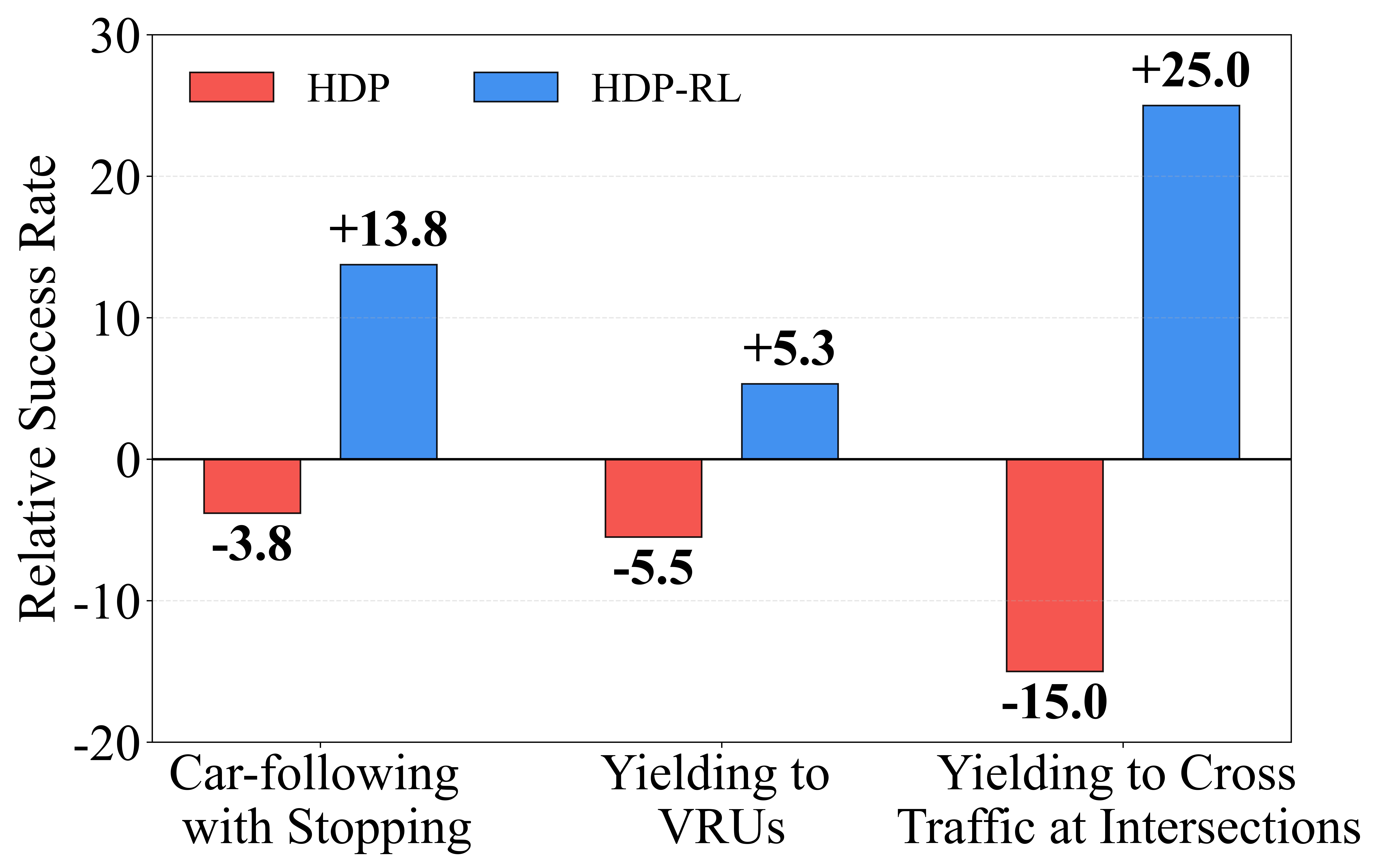
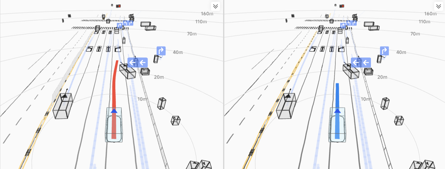
The resulting HDP-RL shows significant improvements in safety-critical scenarios (yielding at intersections, VRU avoidance) while preserving overall driving stability—completing the progression from "it drives" to "it drives safely."
RL improvement

Safety-related success rate improvement after RL post-training.

Case 1 Case 2

Trajectory comparison—red HDP vs. blue HDP-RL (RL steers away from collision).

Theorem — KL-regularized RL = weighted hybrid regression

We formulate the RL post-training as a KL-regularized policy optimization that keeps $\pi^{k}$ close to the reference policy $\pi^{k-1}$:

$\displaystyle\max_{\pi^{k}}\;\mathbb{E}_{s\sim\mathcal{D}}\!\left[\,\mathbb{E}_{a\sim\pi^{k}}[\,r(s,a)\,] \;-\; \tfrac{1}{\beta}\,D_{\mathrm{KL}}\!\big(\pi^{k}\,\|\,\pi^{k-1}\big)\right]$

This admits a closed-form optimum $\pi^{k^{\star}}(a\mid s) \propto \pi^{k-1}(a\mid s)\cdot\exp(\beta\,r(s,a))$. We extract it by a single weighted regression step — the RL-hybrid loss:

$\mathcal{L}_{\text{RL-hybrid}} \;=\; \mathbb{E}_{t,\,\epsilon,\,(s,\,\tau^{\mathbf{v}}_{0})\sim\mathcal{D}}\!\left[\,\exp(\beta\,r)\cdot\lVert\tau^{\mathbf{v};k}_{\theta} - \tau^{\mathbf{v}}_{0}\rVert_{\mathit{P}}^{2}\,\right]$

which simply reweights the IL hybrid loss by an exponential reward — same forward pass, same backward pass.

Remark — Compatibility with the Hybrid Loss

The $\mathit{P}$-norm $\lVert\cdot\rVert_{\mathit{P}}^{2}$ is a Bregman divergence (Section 2), so the weighted regression provably extracts the optimal policy $\pi^{k^{\star}}$. RL post-training therefore shares the same loss geometry as IL pretraining — no distribution shift at switch-over.

Algorithm 2 — RL-Hybrid Loss

def rl_hybrid_loss(r, beta, pred_v, gt_v, W, omega):
    # r    : per-candidate reward
    # beta : temperature
    # pred_v, gt_v, W, omega: same as Algorithm 1

    r_n    = (r - r.mean()) / (r.std() + 1e-6)
    weight = torch.exp(beta * r_n).detach()

    return weight * hybrid_loss(pred_v, gt_v, W, omega)

Reuses hybrid_loss from Algorithm 1: the reward weight is detached so gradients flow only through the hybrid regression, preserving the IL training dynamics.

Remark — Per-state cost: K vs K·T

RL-hybrid: $K$ forward-backwards per state ($K$ candidates, single random $t$). Diffusion-PPO baselines: $K\!\cdot\!T$ forward-backwards — one per transition in the $T$-step denoising MDP. With $T\!=\!50$ this is two orders of magnitude of optimization-cost overhead.

More RL results — multi-reward training curves, DPPO-style baseline comparison, and per-step cost analysis — are available in Appendix E.

Real-Vehicle Testing Results

We evaluate every step of the recipe on real-vehicle road tests across 6 urban driving scenarios and 200 km of closed-loop driving. Each component — τ0-loss, velocity supervision, hybrid loss, data scaling, and RL post-training — delivers measurable, compounding gains.

Model Data Open-Loop
Score
Closed-Loop Score
Success Rate Stability Overall
Base Model M 51.07 15.67 0.00 7.83
w/ τ0-loss & τ0-pred M 75.27 22.84 0.00 11.42
+Velocity Supervision M 84.38 34.72 9.24 21.98
+Hybrid Loss M 85.05 61.88 53.88 57.88
+Data Scaling L 86.07 70.59 59.00 64.79
+Data Scaling (HDP) XL 88.94 71.24 79.53 75.38
+RL w/ safety reward (HDP-RL) 72.89 79.53 76.20
+RL w/ multi-rewards (HDP-RL) 83.49 84.65 84.07

highest score per column. Open-loop scores are evaluated by data replay on held-out test datasets; closed-loop scores are obtained from real-world road testing on a real-vehicle platform.

Efficient lane change frame 1 Efficient lane change frame 2
aEfficient Lane Change
Navigational lane change frame 1 Navigational lane change frame 2
bNavigational Lane Change
Vehicle avoidance frame 1 Vehicle avoidance frame 2
cVehicle Avoidance at Intersection
VRU avoidance frame 1 VRU avoidance frame 2
dVRU Avoidance

Closed-loop real-vehicle testing across four representative scenarios, each illustrated with two key frames.

BibTeX

@article{zheng2026unleash,
  title   = {Unleashing the Potential of Diffusion Models for End-to-End Autonomous Driving},
  author  = {Yinan Zheng and Tianyi Tan and Bin Huang and Enguang Liu and Ruiming Liang
             and Jianlin Zhang and Jianwei Cui and Guang Chen and Kun Ma and Hangjun Ye
             and Long Chen and Ya-Qin Zhang and Xianyuan Zhan and Jingjing Liu},
  journal = {arXiv preprint arXiv:2602.22801},
  year    = {2026}
}